Prediction

The Prediction tab applies a trained model to a new large satellite image, producing a georeferenced segmentation map as a GeoTIFF.

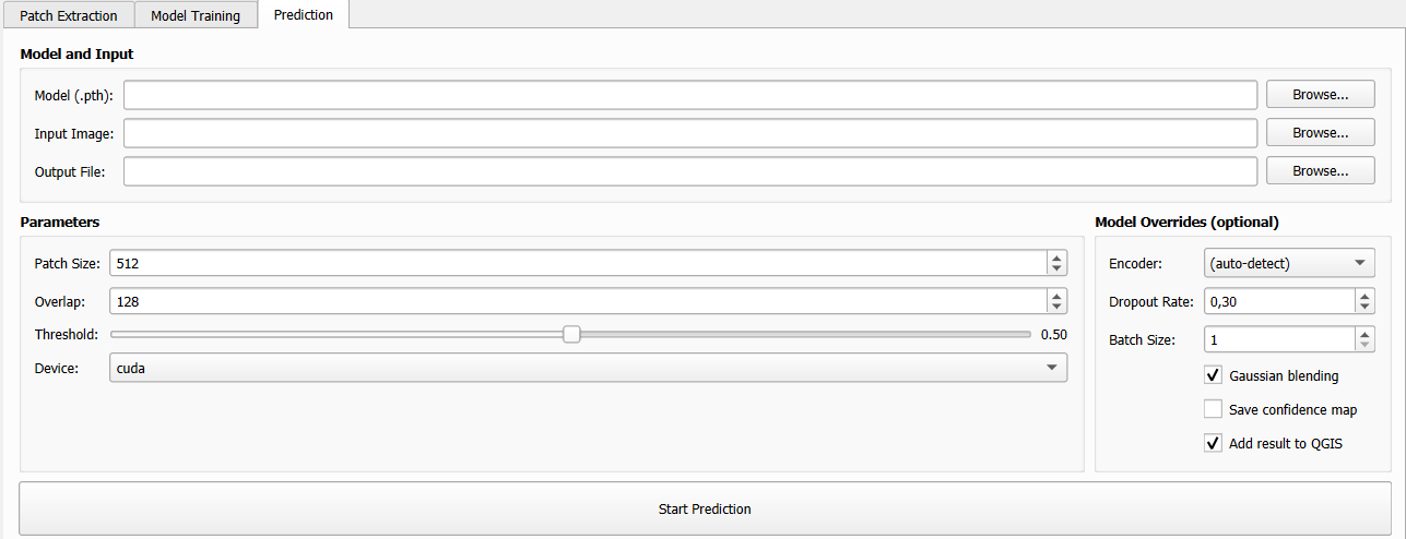
The Prediction tab.

How Prediction Works

Because satellite images are too large to feed directly to a neural network, the prediction engine uses a sliding window approach:

1. The input image is divided into overlapping patches of size Patch Size

2. Each patch is run through the model

3. Predictions are blended back together using Gaussian weighting (optional) to produce a seamless full-resolution output

Sliding window prediction with overlapping patches.

Model and Input Files

Field	Description
Model (.pth)	Path to the trained model checkpoint (.pth file) produced by the Model Training step.
Input Image	Path to the satellite GeoTIFF to segment. Must have the same number of bands as the training data.
Output File	Path for the output segmentation GeoTIFF. The result is a single-band raster with class index values.

Prediction Parameters

Parameters group (left column):

Parameter	Default	Description
Patch Size (px)	512	Size of each inference patch in pixels. Larger patches are faster per pixel but require more GPU memory. Range: 64–2048.
Overlap (px)	128	Number of pixels of overlap between adjacent patches. More overlap → smoother blending but slower inference. Typical values: 64–256.
Threshold	0.50	Decision threshold for binary mode only (0.0–1.0). Pixels with predicted probability above this value are classified as foreground. Has no effect in multi-class mode.
Device	cuda	cuda for GPU inference, cpu for CPU.

Model Override Options (right column)

These optional settings override model metadata read from the checkpoint. Leave them at defaults unless you are using an old checkpoint that lacks metadata.

Parameter	Default	Description
Encoder	(auto-detect)	Override the encoder backbone used during prediction. Leave as (auto-detect) to read the encoder from the checkpoint metadata. Only needed for old checkpoints saved without metadata.
Dropout Rate	0.3	Must match the dropout rate used during training.
Batch Size	1	Number of patches processed simultaneously during inference. Increasing this speeds up GPU inference but uses more memory.
Gaussian blending	checked	Apply Gaussian weighting when merging overlapping patches. Strongly recommended — eliminates visible grid artifacts at patch boundaries.
Save confidence map	unchecked	Additionally save a floating-point GeoTIFF with the raw model output probabilities (binary) or class scores (multi-class).
Add result to QGIS	checked	Automatically load the output segmentation GeoTIFF as a new raster layer in the current QGIS project when prediction completes.

Gaussian Blending

When Gaussian blending is enabled, each overlapping patch is weighted by a 2D Gaussian kernel before being merged into the final image. This means:

• The centre of each patch contributes more than the edges

• Abrupt transitions between patches are smoothed out

• The final result has no visible “grid” pattern

Gaussian blending is always recommended unless you specifically need hard patch boundaries.

Output Format

The output segmentation is a georeferenced single-band GeoTIFF with:

• The same spatial extent, CRS, and pixel resolution as the input image

• Integer pixel values representing class indices: - 0 / 1 for binary mode (background / foreground) - 0, 1, 2, … for multi-class mode

If Save confidence map is checked, a second file is saved alongside the classification result with the suffix _confidence.tif, containing floating-point values in the range [0, 1].

When Add result to QGIS is checked, the output is automatically added as a raster layer to the current project with a default style. You can then apply your own colour ramp in the layer properties.

Tips for Good Predictions

Match training resolution

Ensure the input image has the same spatial resolution as the images used during training. Feeding a 10m image to a model trained on 30m data will produce poor results.

Match the number of bands

The input image must have the same number of bands (channels) as the images used during training. The model was trained on a specific band configuration; mismatches will cause an error.

Patch Size vs. Overlap trade-offs

Patch Size	Overlap	Characteristics
256	64–128	Low memory, faster
512	128–256	Balanced (default)
1024	256–512	Slow, high VRAM, best for textures

GPU out of memory

If you encounter CUDA out-of-memory errors:

1. Reduce Patch Size (e.g., from 512 to 256)

2. Reduce Batch Size to 1

3. Switch Device to cpu (slower but unlimited memory)

Prediction Log

During prediction, the output panel reports:

Loading model from: /path/to/best_model.pth
Architecture: unet | Encoder: resnet34 | Mode: binary
Input image: 10000×8000 px, 4 bands
Processing 256 patches (16×16 grid)...
[██████████████████░░░░] 72% (185/256 patches)
Prediction complete!
Output saved to: /path/to/output_segmentation.tif
Layer added to QGIS: output_segmentation