Tutorial: Land Cover Classification from BD Ortho IRC

This step-by-step tutorial walks you through a complete workflow — from raw data to a classified map — using SemanticSeg4EO. It is designed as a starting point to help you get familiar with the tool.

All data used and produced in this tutorial (raw imagery, labels, grid, extracted patches, trained model and predictions) are freely available on Zenodo:

📦 Dataset & results: https://zenodo.org/records/18784043

Input Data

This tutorial uses the following inputs:

Input	Description
Satellite image	BD Ortho at 20 cm resolution, IRC (Infrared–Red–Green) composite — 3 bands
Labels	Land cover mask derived from OCS GE, 5 classes (values 0 to 4)
Grid	Polygon shapefile defining the patch locations over the study area

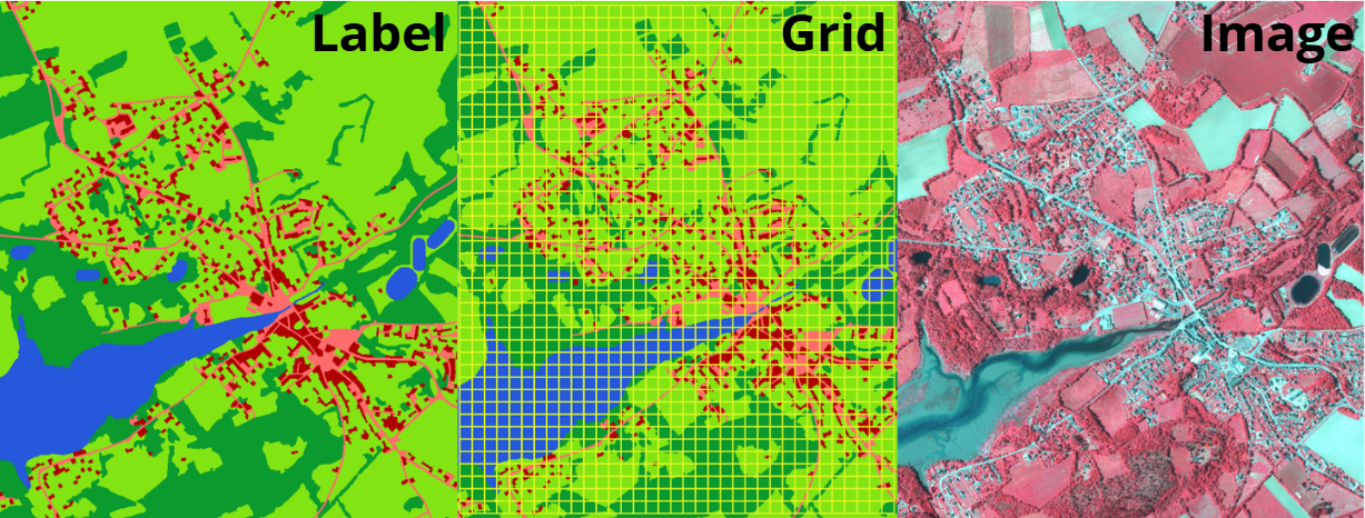
Overview of the input data loaded in QGIS: BD Ortho IRC image, OCS GE labels, and the extraction grid.

Step 1 — Patch Extraction

Open SemanticSeg4EO and navigate to the Patch Extraction tab.

Select the input files:

• Satellite Image: the BD Ortho IRC GeoTIFF

• Labels / Mask: the OCS GE raster (5 classes, 0–4)

• Grid: the polygon shapefile

Set the extraction parameters:

Patch size	224
Image channels	3 (IRC)
Data type	int16
Train / Val / Test ratio	0.70 / 0.20 / 0.10

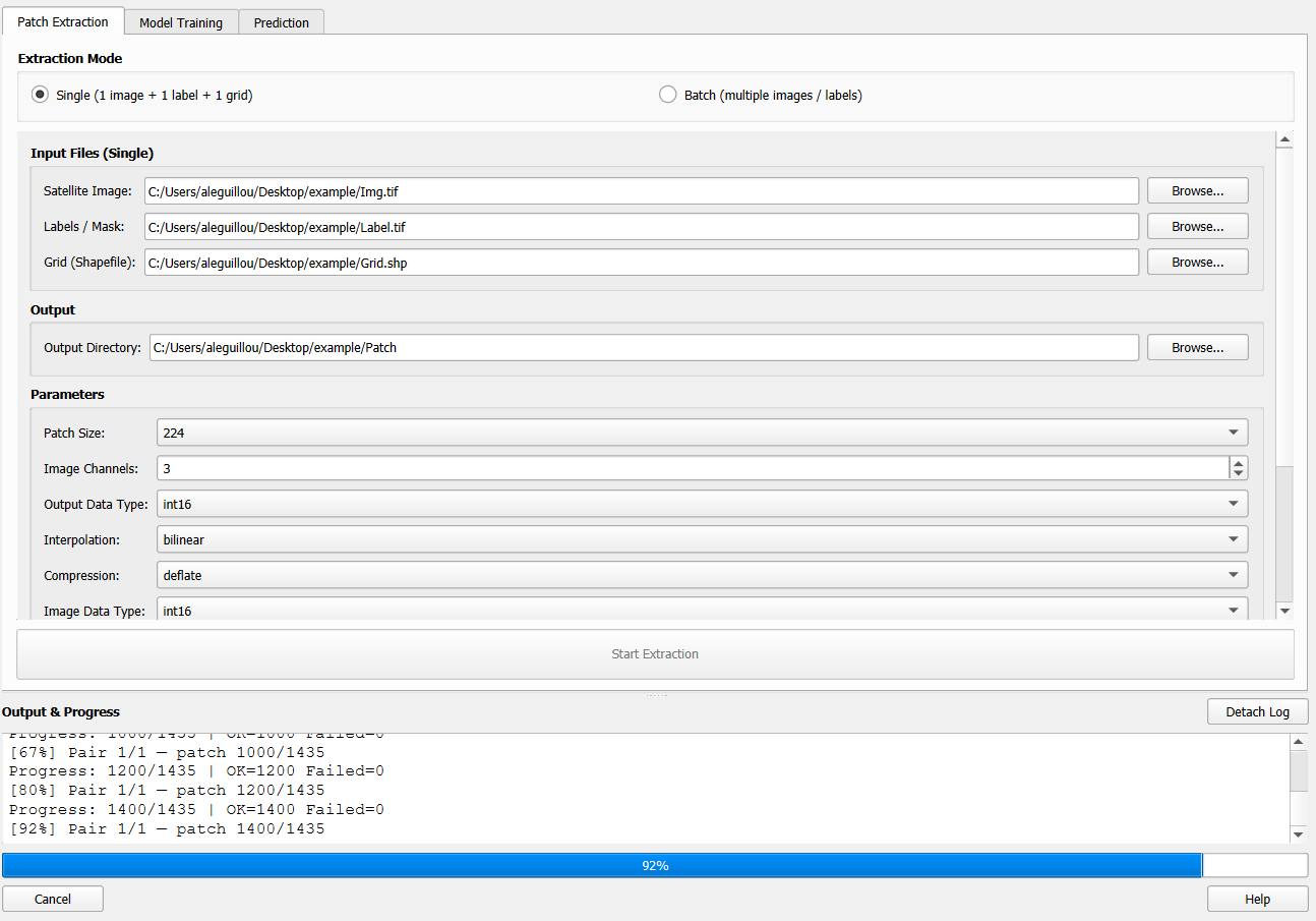
Patch extraction tab with the parameters used in this tutorial.

Click Run Extraction. The plugin extracts 1 435 patches into the output directory, organised as follows:

output_dir/
└── Patch/
    ├── train/
    │   ├── images/    (1 076 patches)
    │   └── labels/
    ├── validation/
    │   ├── images/    (215 patches)
    │   └── labels/
    └── test/
        ├── images/    (144 patches)
        └── labels/

Each patch is a georeferenced GeoTIFF that can be loaded directly in QGIS for visual inspection.

Step 2 — Model Training

Navigate to the Model Training tab.

Select the dataset:

• Dataset directory: the Patch/ folder created in Step 1

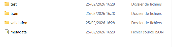
The Patch folder containing train, validation and test splits.

Configure the training:

Mode	Multi-class
Number of classes	5
Architecture	U-Net
Encoder	Resnet-34
Epochs	as needed (see training curves)
Device	cuda (GPU) or cpu

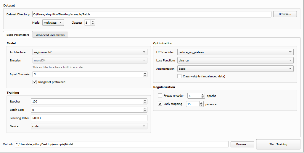
Model training tab configured for U-Net + Resnet-34, multi-class (5 classes).

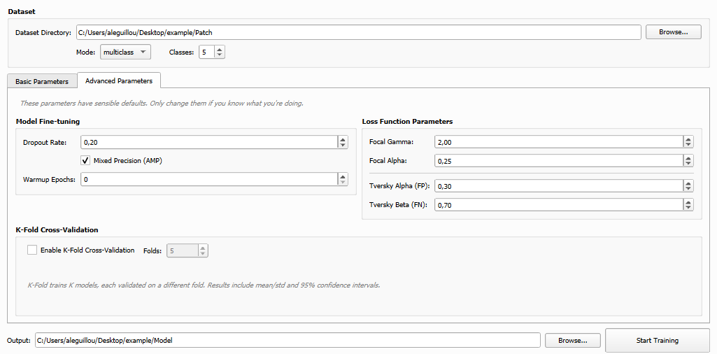
Advanced training parameters.

Click Run Training. The plugin launches the training in the external environment. Progress and metrics are displayed in the log panel.

Once training is complete, the output directory contains:

trained_models/
├── model_best_iou.pth           ← best IoU checkpoint
├── model_best_loss.pth          ← best validation loss checkpoint
├── model_final_model.pth        ← final model weights
├── model_metrics.json           ← detailed metrics history
└── model_training_plot.png      ← training curves

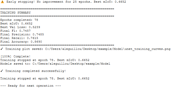
Training results: metrics summary and training curves.

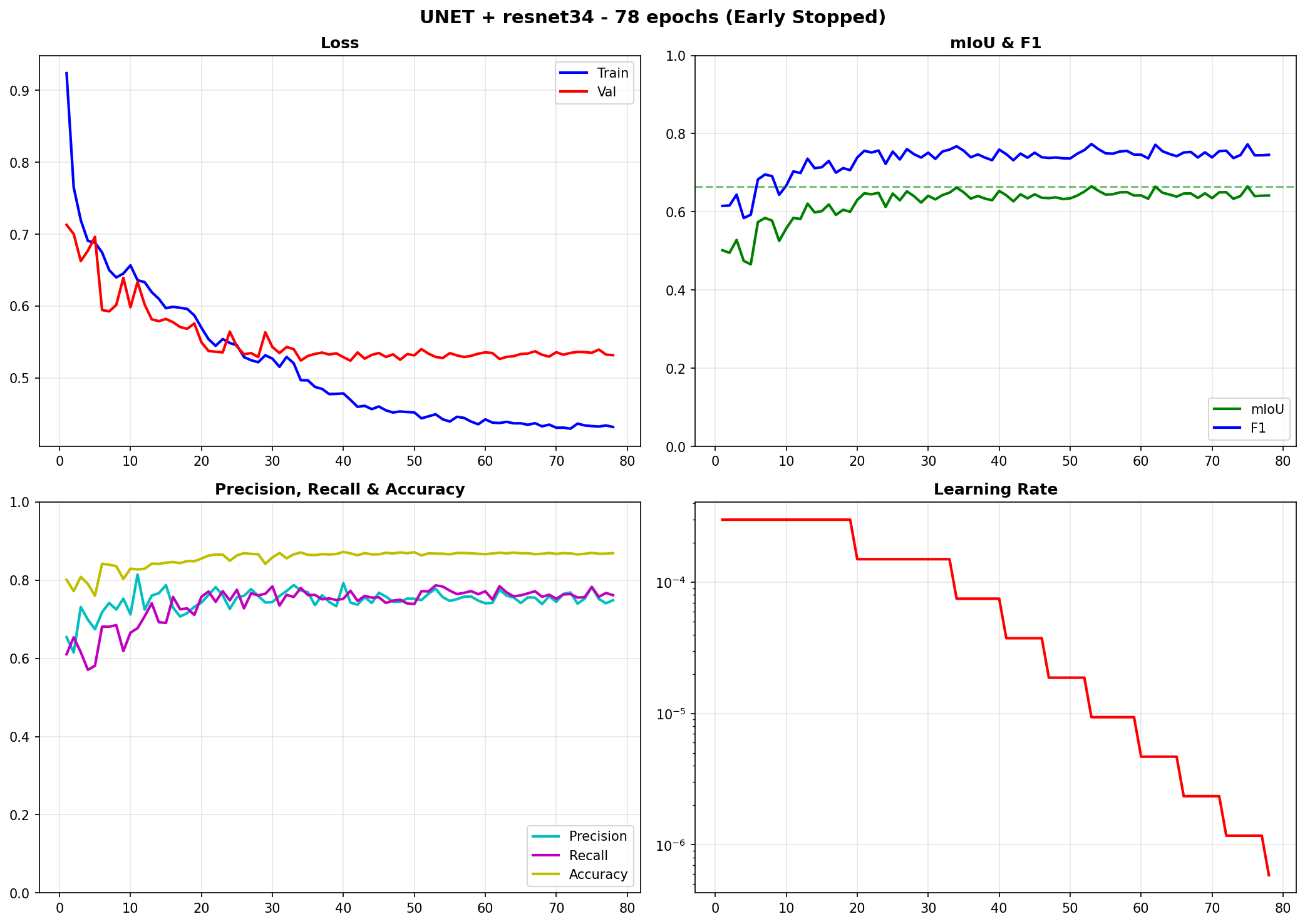
Loss and IoU curves over the training epochs.

Warning

The results presented in this tutorial were obtained using a small subset (1 405 patches of 224 × 224 × 3 pixels) for demonstration purposes only. Performance can be substantially improved by:

• Increasing the training area — adding more images and labels to provide the model with a larger and more diverse set of training pixels

• Tuning hyperparameters — adjusting learning rate, batch size, scheduler, loss function, augmentation level, etc.

• Trying different architectures or encoders — e.g. switching from SegFormer-B2 to a larger variant, or using a pretrained ResNet-101 backbone

• Enabling advanced options — class weighting, k-fold cross-validation, mixed-precision training, or stronger data augmentation

This tutorial is intended as a starting point to familiarise yourself with the SemanticSeg4EO workflow, not as an optimised benchmark.

Step 3 — Prediction on an Independent Image

To evaluate the generalisation ability of the model, we apply it to an independent image that was not used during training. This image has the same characteristics as the training data: BD Ortho at 20 cm resolution, IRC composite.

Navigate to the Prediction tab and configure:

• Model: the .pth file from Step 2 (e.g. model_best_iou.pth)

• Input image: the independent BD Ortho IRC scene

• Output: path for the prediction GeoTIFF

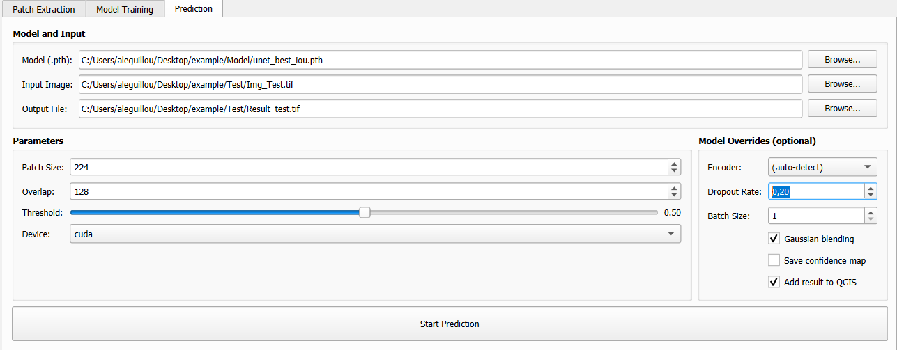
Prediction tab: model, independent input image and output path.

Click Run Prediction. The plugin performs patch-based inference with seamless reconstruction.

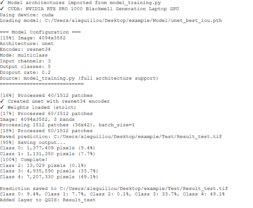
Results of logs after predictions.

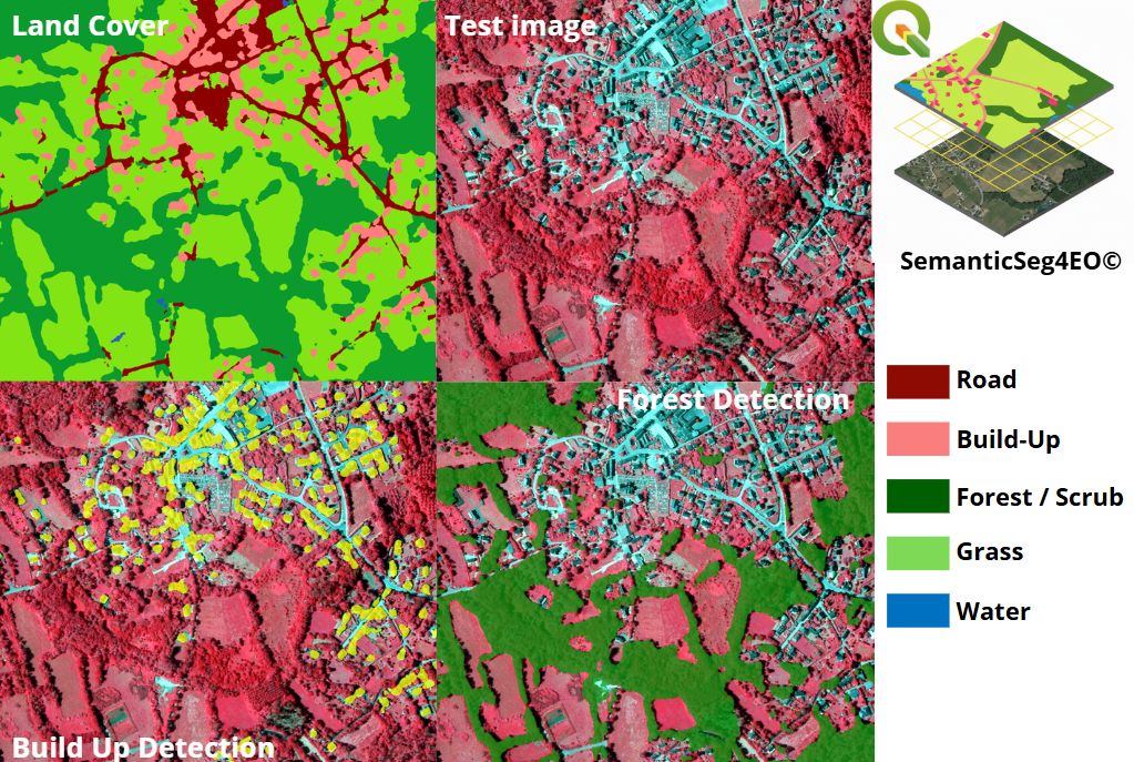
Prediction result on the independent image, displayed in QGIS alongside the original BD Ortho IRC.

Summary

This tutorial covered the three main steps of a SemanticSeg4EO workflow:

1. Patch extraction — preparing a training dataset from large satellite imagery

2. Model training — training a SegFormer-B2 on 5 land cover classes

3. Prediction — applying the trained model to a new, unseen image

The numerical scores (IoU, F1, accuracy) provide a quantitative assessment of model performance, while the visual prediction on an independent scene demonstrates the model’s ability to generalise beyond the training area.

Note

All data (BD Ortho IRC images, OCS GE labels, grid shapefile, extracted patches, trained model, and predictions) are freely available for download on Zenodo so that you can reproduce this tutorial exactly:

📦 https://zenodo.org/records/18784043